Mastering Waterfall Charts In Excel: A Complete Information

Mastering Waterfall Charts in Excel: A Complete Information

Associated Articles: Mastering Waterfall Charts in Excel: A Complete Information

Introduction

On this auspicious event, we’re delighted to delve into the intriguing matter associated to Mastering Waterfall Charts in Excel: A Complete Information. Let’s weave attention-grabbing data and provide contemporary views to the readers.

Mastering Waterfall Charts in Excel: A Complete Information

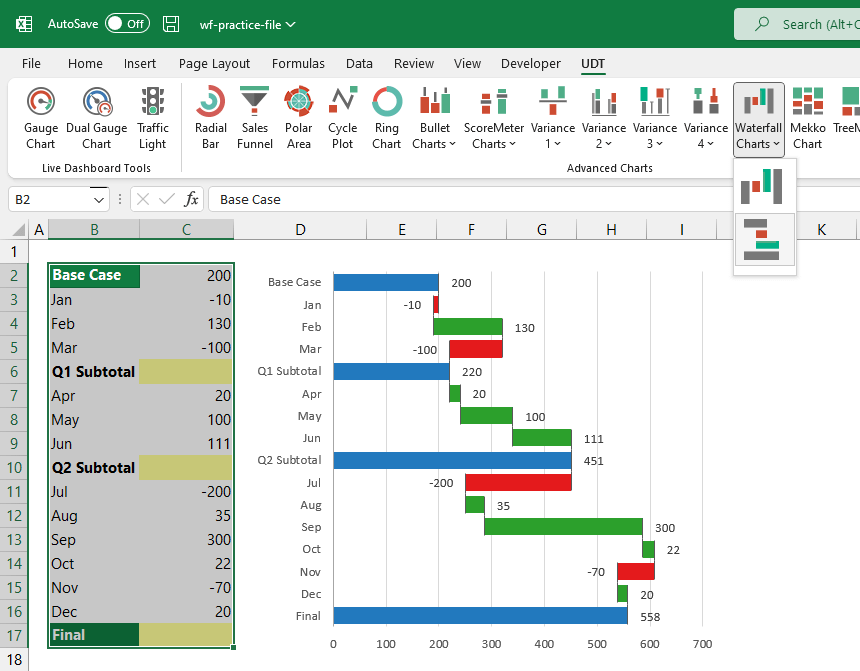
Waterfall charts, often known as bridge charts or flying bricks charts, are highly effective visible instruments for showcasing the cumulative impact of constructive and adverse adjustments over time or throughout classes. In contrast to conventional bar charts, which merely show particular person values, waterfall charts clearly illustrate how an preliminary worth is modified by a sequence of incremental will increase and reduces, finally resulting in a remaining worth. This makes them ultimate for demonstrating monetary efficiency, useful resource allocation, mission budgeting, and numerous different situations requiring a transparent visualization of sequential adjustments. This text offers a complete information to creating efficient waterfall charts in Excel, overlaying each handbook strategies and leveraging Excel’s built-in options (out there in newer variations).

I. Understanding the Elements of a Waterfall Chart:

Earlier than diving into the creation course of, let’s perceive the important thing parts:

• Beginning Worth: The preliminary worth from which the adjustments originate. That is often the primary bar within the chart.
• Optimistic Adjustments (Will increase): These are represented by bars extending upwards from the earlier worth.
• Detrimental Adjustments (Decreases): These are represented by bars extending downwards from the earlier worth.
• Intermediate Values: The values ensuing after every constructive or adverse change. These are implicitly represented by the peak of the bars at every stage.
• Ending Worth: The ultimate worth in any case adjustments have been integrated. That is the peak of the final bar.

II. Making a Waterfall Chart Manually in Excel (Older Variations):

For Excel variations missing built-in waterfall chart performance, a handbook method is important. This entails cautious information structuring and using stacked bar charts:

1. Knowledge Preparation:

Set up your information in a desk with the next columns:

• Class: Describes every change (e.g., "Beginning Steadiness," "Gross sales," "Bills," "Revenue").
• Worth: The numerical worth of every change. Optimistic values signify will increase, and adverse values signify decreases.

Instance:

Class	Worth
Beginning Steadiness	10000
Gross sales	5000
Price of Items Bought	-2000
Working Bills	-1500
Internet Revenue	1500

2. Calculating Intermediate Values:

Add a brand new column "Working Complete" to calculate the cumulative worth after every change. The formulation for the second row onwards might be: =Earlier Row's Working Complete + Present Row's Worth.

Class	Worth	Working Complete
Beginning Steadiness	10000	10000
Gross sales	5000	15000
Price of Items Bought	-2000	13000
Working Bills	-1500	11500
Internet Revenue	1500	13000

3. Creating the Stacked Bar Chart:

• Choose the "Class" and "Working Complete" columns.
• Go to "Insert" -> "Chart" -> "Column" -> "Stacked Column".
• It will create a stacked bar chart. Nonetheless, it will not but appear to be a waterfall chart.

4. Adjusting the Chart for Waterfall Look:

• Detrimental Bars: Proper-click on the adverse bars (these representing decreases). Choose "Format Knowledge Collection." Below "Collection Choices," change the "Collection Overlap" to 100% and the "Hole Width" to 0%. It will make sure the adverse bars lengthen downwards seamlessly.
• Optimistic Bars: Regulate the fill coloration of the constructive bars to distinguish them visually from the adverse bars.
• Formatting: Add information labels to show the values of every change. That is essential for readability. You may want to regulate label positions for optimum readability.
• Axis: Regulate the vertical axis to begin at zero or a related minimal worth for a greater visible illustration.

III. Making a Waterfall Chart utilizing Excel’s Constructed-in Function (Newer Variations):

Excel variations 2013 and later provide a built-in waterfall chart sort, simplifying the method considerably:

1. Knowledge Preparation:

Put together your information as described within the handbook methodology (Class and Worth columns). You do not want the "Working Complete" column for this methodology.

2. Inserting the Waterfall Chart:

• Choose your information (Class and Worth columns).
• Go to "Insert" -> "Chart" -> "Different Charts" -> "Waterfall".
• Excel will routinely generate a waterfall chart.

3. Chart Customization:

• Labels: Add information labels to show values for readability.
• Colours: Regulate the colours of constructive and adverse bars for higher visible distinction.
• Axis: Regulate the vertical axis to begin at zero or an appropriate minimal worth.
• **

Closure

Thus, we hope this text has supplied priceless insights into Mastering Waterfall Charts in Excel: A Complete Information. We thanks for taking the time to learn this text. See you in our subsequent article!