Mastering The Ggplot2 Donut Chart: A Complete Information

Mastering the ggplot2 Donut Chart: A Complete Information

Associated Articles: Mastering the ggplot2 Donut Chart: A Complete Information

Introduction

On this auspicious event, we’re delighted to delve into the intriguing matter associated to Mastering the ggplot2 Donut Chart: A Complete Information. Let’s weave attention-grabbing data and supply recent views to the readers.

Mastering the ggplot2 Donut Chart: A Complete Information

The donut chart, a visually interesting variation of the pie chart, provides a superb technique to signify proportions of a categorical variable. Whereas pie charts can typically be tough to interpret precisely, notably when coping with many classes or closely-spaced proportions, donut charts usually enhance readability by including a central house, permitting for added data or a extra visually balanced presentation. Within the realm of knowledge visualization with R, the ggplot2 package deal gives a robust and versatile framework for creating gorgeous and informative donut charts. This text will delve into the creation of those charts utilizing ggplot2, overlaying numerous customization choices and superior strategies.

Fundamentals: Constructing a Primary Donut Chart

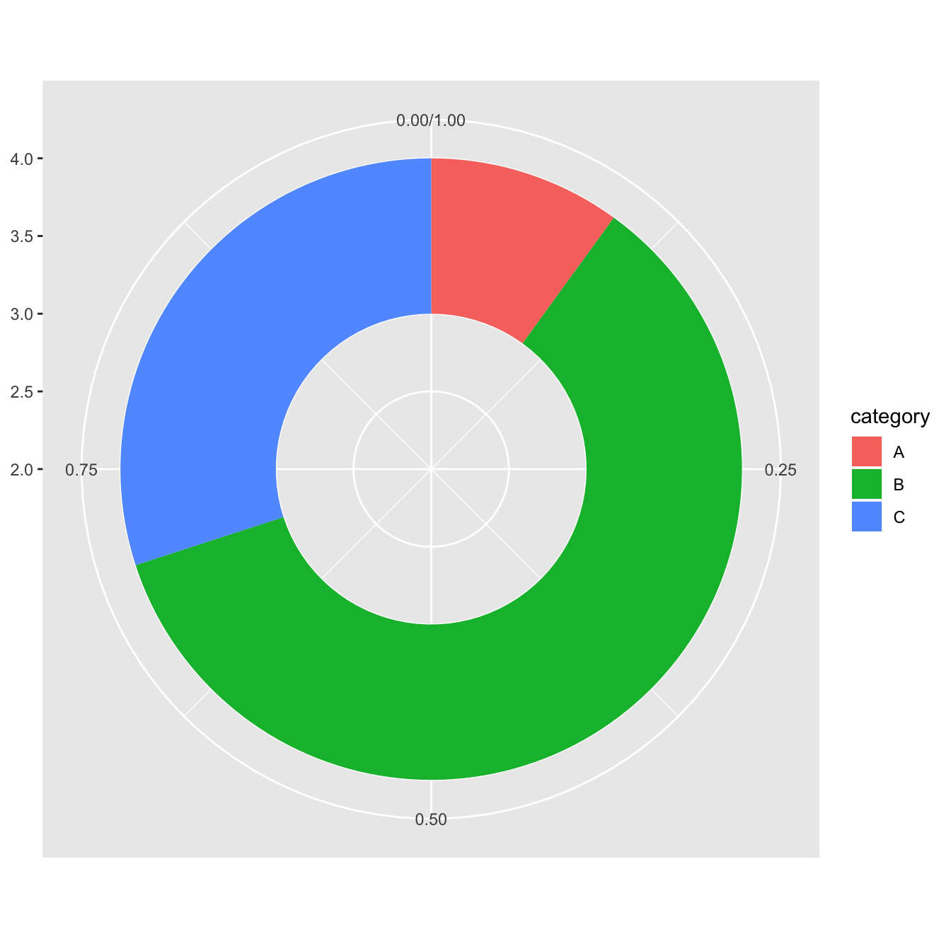
The inspiration of any ggplot2 chart lies within the ggplot() perform, which initializes the plot. We then layer on completely different geometric objects (geom_) and aesthetic mappings (aes()). For a donut chart, we primarily use geom_col() (for creating the segments) and coord_polar() (for reworking the bar chart right into a circle).

Let’s think about a easy instance: suppose we’ve got information available on the market share of various cellular working programs:

library(ggplot2)

information <- information.body(
  OS = c("Android", "iOS", "Home windows", "Different"),
  MarketShare = c(0.7, 0.25, 0.03, 0.02)
)

A primary donut chart will be created as follows:

ggplot(information, aes(x = "", y = MarketShare, fill = OS)) +
  geom_col(width = 1, colour = "white") +
  coord_polar("y", begin = 0) +
  theme_void() +
  labs(fill = "Working System") +
  ggtitle("Cell OS Market Share")

This code first creates a ggplot object with the information, mapping the MarketShare to the y-axis (which determines phase measurement) and OS to the fill colour. geom_col() creates the bars, with width = 1 making certain they kind an entire circle. coord_polar("y", begin = 0) transforms the bars right into a circle, beginning on the 0 diploma mark. theme_void() removes pointless axes and gridlines, and labs() and ggtitle() add labels and a title.

Enhancing the Visible Enchantment: Customization Choices

The essential donut chart gives a purposeful illustration, however ggplot2 permits for intensive customization to reinforce its visible attraction and data density.

• Shade Palette: The default colour palette may not all the time be superb. ggplot2 provides a number of built-in palettes (e.g., scale_fill_brewer(), scale_fill_viridis_d()), or you may specify customized colours utilizing vectors. For instance, utilizing a viridis palette:

ggplot(information, aes(x = "", y = MarketShare, fill = OS)) +
  geom_col(width = 1, colour = "white") +
  coord_polar("y", begin = 0) +
  scale_fill_viridis_d() +
  theme_void() +
  labs(fill = "Working System") +
  ggtitle("Cell OS Market Share")

• Including Labels: Displaying percentages inside every phase improves readability. We are able to calculate percentages and add them utilizing geom_text():

information$Share <- spherical(information$MarketShare * 100, 1)
ggplot(information, aes(x = "", y = MarketShare, fill = OS)) +
  geom_col(width = 1, colour = "white") +
  geom_text(aes(label = paste0(Share, "%")), place = position_stack(vjust = 0.5)) +
  coord_polar("y", begin = 0) +
  scale_fill_viridis_d() +
  theme_void() +
  labs(fill = "Working System") +
  ggtitle("Cell OS Market Share")

• Central Textual content: The central house can be utilized to show extra data, corresponding to a title or abstract statistic. This may be achieved utilizing annotate():

ggplot(information, aes(x = "", y = MarketShare, fill = OS)) +
  geom_col(width = 1, colour = "white") +
  geom_text(aes(label = paste0(Share, "%")), place = position_stack(vjust = 0.5)) +
  coord_polar("y", begin = 0) +
  scale_fill_viridis_d() +
  annotate("textual content", x = 0, y = 0, label = "Complete Market Share", measurement = 8) +
  theme_void() +
  labs(fill = "Working System") +
  ggtitle("Cell OS Market Share")

• Legend Customization: The legend will be additional custom-made utilizing capabilities like theme(legend.place = "backside") to put it on the backside, or theme(legend.title = element_text(measurement = 12)) to regulate the title’s measurement.

Dealing with Bigger Datasets and Advanced Situations

The strategies described above work properly for smaller datasets. For bigger datasets with many classes, cautious consideration is required to keep away from visible litter. Methods embody:

• Grouping Classes: When you’ve got many classes, think about grouping them into broader classes to cut back the variety of segments.

• Interactive Charts: For very massive datasets, think about using interactive charting libraries like plotly to permit customers to discover the information extra successfully. ggplotly() from the plotly package deal can simply convert a ggplot2 chart into an interactive one.

• Highlighting Key Segments: Use colour and measurement to emphasise notably vital segments.

Past the Fundamentals: Superior Methods

ggplot2‘s flexibility extends past primary donut charts. We are able to create extra subtle visualizations:

• Donut Charts with A number of Rings: Representing a number of variables utilizing concentric rings creates a richer visualization. This requires cautious information manipulation and layering of geom_col() objects.

• Animated Donut Charts: Utilizing packages like gganimate, we are able to create animated donut charts that present modifications in proportions over time.

• Customized Shapes: Whereas round is the norm, you may experiment with completely different shapes utilizing customized coordinate programs.

Conclusion

ggplot2 gives a strong and versatile atmosphere for creating visually interesting and informative donut charts. By mastering the core rules and exploring the customization choices, you may successfully talk advanced information utilizing this versatile chart sort. Bear in mind to contemplate your viewers and the particular message you want to convey when choosing the suitable customizations and superior strategies. The secret is to create a chart that’s each visually partaking and simply interpretable, making certain your information insights are clearly communicated. This complete information has supplied a robust basis to your journey in creating impactful donut charts with ggplot2, encouraging you to discover the huge potentialities inside this highly effective information visualization framework. Via experimentation and additional exploration of the ggplot2 documentation, it is possible for you to to craft extremely custom-made and informative donut charts to fit your particular information evaluation wants.

Closure

Thus, we hope this text has supplied priceless insights into Mastering the ggplot2 Donut Chart: A Complete Information. We respect your consideration to our article. See you in our subsequent article!