Mastering Stacked Space Charts In R With Ggplot2: A Complete Information

Mastering Stacked Space Charts in R with ggplot2: A Complete Information

Associated Articles: Mastering Stacked Space Charts in R with ggplot2: A Complete Information

Introduction

With nice pleasure, we are going to discover the intriguing subject associated to Mastering Stacked Space Charts in R with ggplot2: A Complete Information. Let’s weave fascinating info and supply contemporary views to the readers.

Mastering Stacked Space Charts in R with ggplot2: A Complete Information

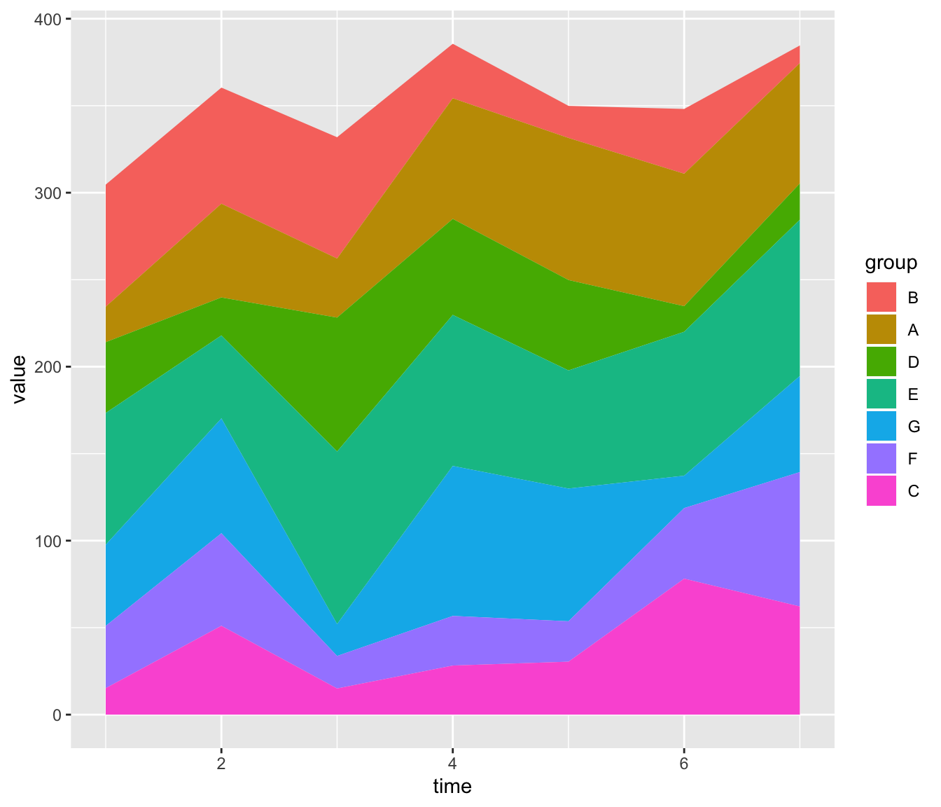
Stacked space charts are highly effective visualization instruments used to show the composition of a complete over time or throughout classes. They’re notably efficient at exhibiting the relative contribution of various components to a complete, revealing developments and patterns that could be missed in different chart sorts. R, coupled with the versatile ggplot2 package deal, gives a strong and stylish framework for creating compelling stacked space charts. This text delves deep into the creation and customization of those charts, overlaying all the pieces from fundamental implementation to superior strategies for enhancing readability and conveying insights successfully.

Fundamentals: Setting up a Fundamental Stacked Space Chart

Earlier than diving into intricate customizations, let’s set up a basis by setting up a fundamental stacked space chart. We’ll use a pattern dataset for demonstration. We could say we’ve got information on the gross sales of three totally different product traces (A, B, and C) over a five-year interval:

library(ggplot2)

# Pattern information
information <- information.body(
  Yr = rep(2018:2022, every = 3),
  Product = issue(rep(c("A", "B", "C"), 5)),
  Gross sales = c(10, 15, 20, 12, 18, 25, 15, 22, 30, 18, 25, 35)
)

Now, let’s create the essential stacked space chart utilizing ggplot2:

ggplot(information, aes(x = Yr, y = Gross sales, fill = Product)) +
  geom_area() +
  labs(title = "Product Gross sales Over Time",
       x = "Yr",
       y = "Gross sales",
       fill = "Product Line")

This code snippet generates a stacked space chart the place the x-axis represents the yr, the y-axis represents gross sales, and the totally different coloured areas characterize the gross sales of every product line. The fill aesthetic maps the Product variable to the fill coloration of every space. The labs() operate provides a title and axis labels for readability.

Enhancing Visible Attraction and Readability

Whereas the essential chart is purposeful, a number of enhancements can enhance its readability and aesthetic attraction.

• Colour Palette: The default coloration palette may not all the time be optimum. ggplot2 provides numerous palettes, or you need to use customized palettes from packages like RColorBrewer or viridis.

ggplot(information, aes(x = Yr, y = Gross sales, fill = Product)) +
  geom_area(aes(coloration = Product)) + # add borders for higher distinction
  scale_fill_brewer(palette = "Set3") + # use a brewer palette
  scale_color_brewer(palette = "Set3") +
  labs(title = "Product Gross sales Over Time",
       x = "Yr",
       y = "Gross sales",
       fill = "Product Line") +
  theme_bw() # use a black and white theme

• Including Labels and Annotations: Including labels on to the chart can spotlight key information factors or developments. The geom_text() operate is helpful for this function. Nevertheless, cautious placement is essential to keep away from cluttering the chart.

• Axis Limits and Breaks: Adjusting axis limits and breaks can enhance the visible illustration of the info. The scale_x_continuous() and scale_y_continuous() features permit for exact management.

• Theme Customization: ggplot2 provides numerous themes (theme_bw(), theme_minimal(), and so forth.) to change the general look of the chart. It’s also possible to customise particular person theme parts for granular management.

• Legends: The legend is essential for understanding the chart’s parts. You possibly can modify its place, title, and key utilizing theme() and legend.place.

Dealing with Lacking Knowledge and Knowledge Transformation

Actual-world datasets typically include lacking information. ggplot2 handles lacking information gracefully, however understanding its implications is crucial. Lacking information can result in gaps within the stacked space chart. Contemplate imputation strategies or cautious information cleansing to handle lacking values.

Knowledge transformations, comparable to logarithmic scales, could be obligatory for datasets with skewed distributions or broad ranges of values. scale_y_log10() can be utilized to use a logarithmic transformation to the y-axis.

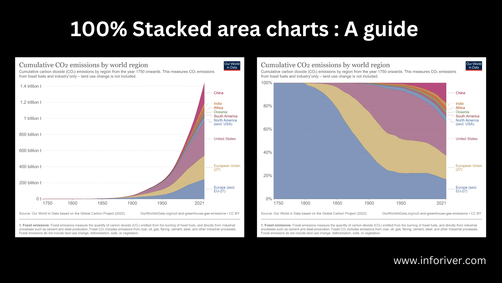
Superior Strategies: % Stacked Space Charts and Faceting

• % Stacked Space Charts: As an alternative of exhibiting absolute values, it is typically extra insightful to show the relative contribution of every part. That is achieved by calculating percentages earlier than plotting.

data_percent <- information %>%
  group_by(Yr) %>%
  mutate(% = Gross sales / sum(Gross sales) * 100)

ggplot(data_percent, aes(x = Yr, y = %, fill = Product)) +
  geom_area() +
  scale_y_continuous(labels = scales::p.c) +
  labs(title = "Product Gross sales Proportion Over Time",
       x = "Yr",
       y = "Gross sales Proportion",
       fill = "Product Line")

• Faceting: For datasets with a number of classes or grouping variables, faceting permits for displaying a number of stacked space charts in a grid, enhancing comparability and revealing interactions between variables. The facet_wrap() or facet_grid() features are used for faceting.

Troubleshooting and Greatest Practices

• Overplotting: With many classes or densely packed information, the chart may change into cluttered. Think about using fewer classes, aggregating information, or using different visualization strategies.

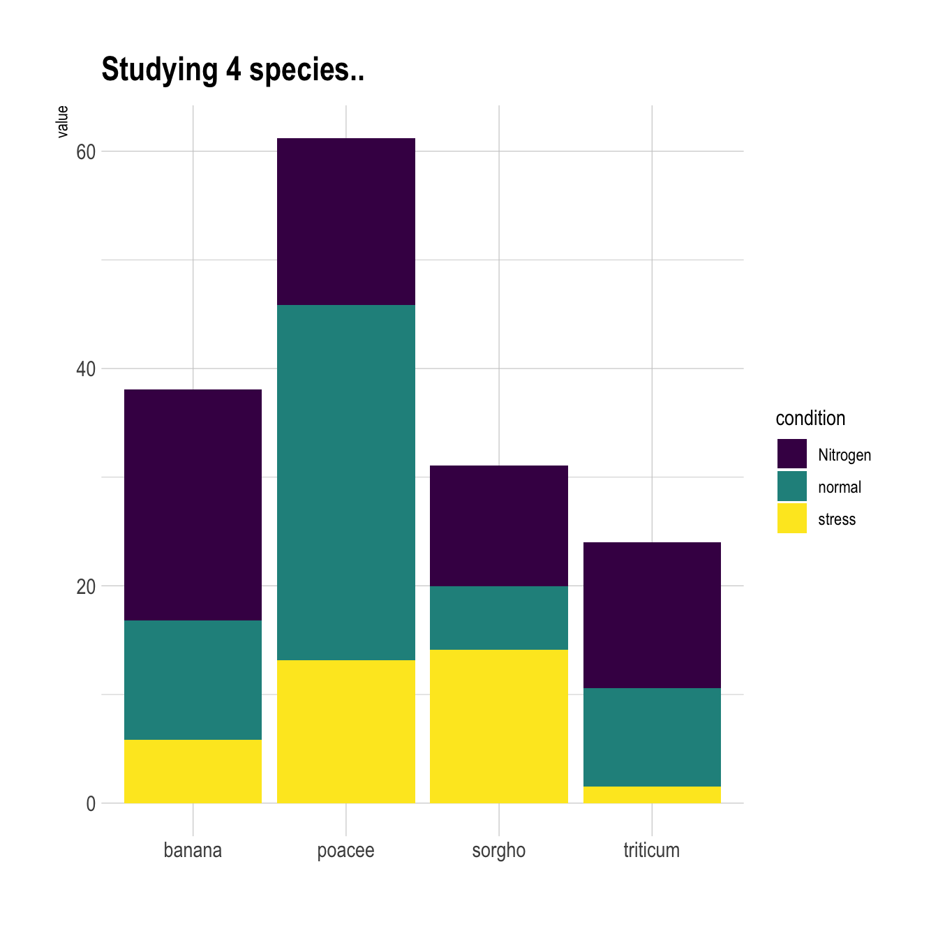
• Knowledge Ordering: The order of the stacked areas influences the visible notion. Make sure the order is logical and significant. You possibly can management the order utilizing issue() to reorder the degrees of the fill variable.

• Accessibility: Contemplate accessibility for customers with visible impairments. Use clear and contrasting colours, present descriptive labels, and guarantee enough distinction between textual content and background.

Conclusion:

Stacked space charts, when applied successfully, present a robust strategy to visualize the composition of a complete over time or throughout classes. ggplot2 in R provides a versatile and stylish framework for creating these charts, permitting for intensive customization to boost readability, visible attraction, and insightful information communication. By mastering the strategies outlined on this article, you’ll be able to create compelling and informative stacked space charts that successfully talk advanced information patterns and developments. Keep in mind to all the time think about your viewers and the precise insights you intention to convey when designing your visualizations. Via cautious planning, information preparation, and considerate software of ggplot2‘s capabilities, you’ll be able to unlock the complete potential of stacked space charts for information storytelling.

Closure

Thus, we hope this text has offered invaluable insights into Mastering Stacked Space Charts in R with ggplot2: A Complete Information. We thanks for taking the time to learn this text. See you in our subsequent article!