Mastering Pie Charts In Excel: A Complete Information From A Single Column Of Information

Mastering Pie Charts in Excel: A Complete Information from a Single Column of Information

Associated Articles: Mastering Pie Charts in Excel: A Complete Information from a Single Column of Information

Introduction

On this auspicious event, we’re delighted to delve into the intriguing matter associated to Mastering Pie Charts in Excel: A Complete Information from a Single Column of Information. Let’s weave attention-grabbing info and supply recent views to the readers.

Mastering Pie Charts in Excel: A Complete Information from a Single Column of Information

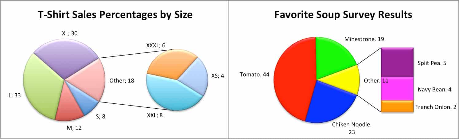
Pie charts, with their visually interesting round segments, supply a robust method to symbolize proportional information. They’re notably efficient for showcasing the relative contribution of various classes to an entire. Whereas Excel affords strong charting capabilities, making a compelling pie chart from a single column of information can generally really feel daunting, particularly with massive datasets. This complete information will stroll you thru the method step-by-step, protecting numerous eventualities and offering superior ideas for optimizing your charts for readability and influence.

Understanding the Conditions: Your Single Column Information

Earlier than we dive into chart creation, let’s make clear what we imply by "a single column of information." This refers to a state of affairs the place your information is organized with:

• One column containing class labels: This column lists the totally different classes you wish to symbolize in your pie chart (e.g., product names, areas, age teams).
• One other column (optionally available however extremely advisable) containing the corresponding values: This column supplies the numerical information representing the scale or frequency of every class. If you happen to solely have the class labels, Excel can nonetheless create a pie chart, however it’ll assume equal proportions for every class.

Situation 1: Information in Two Columns (Preferrred Situation)

That is essentially the most easy state of affairs. Let’s assume you’ve:

• Column A: Class Labels (e.g., "Apples," "Bananas," "Oranges")
• Column B: Corresponding Values (e.g., 100, 150, 50)

Steps to Create the Pie Chart:

1. Choose your information: Spotlight each Column A and Column B, together with the header row (when you have one). Guarantee your choice kinds an oblong block.

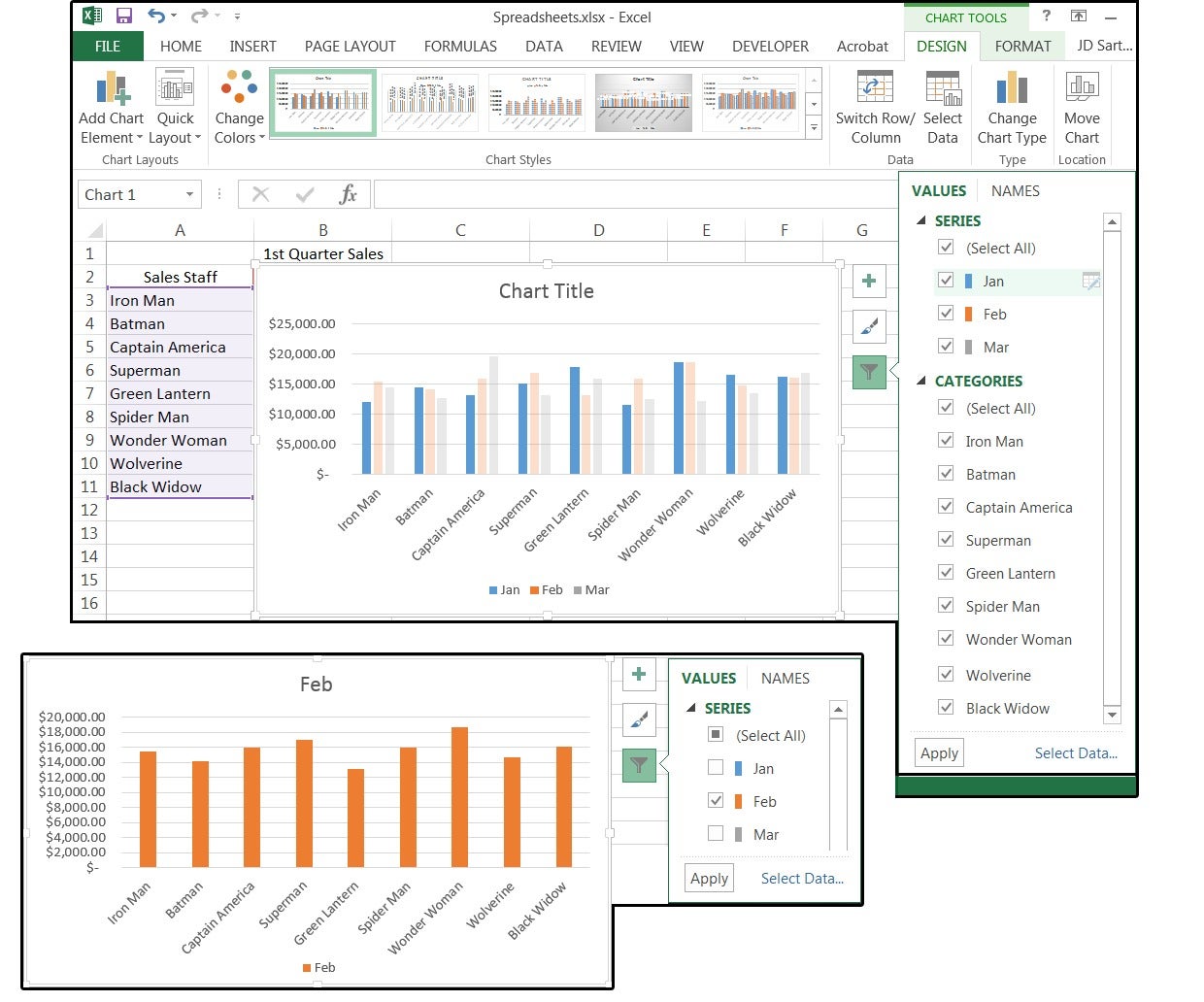
2. Insert a Pie Chart: Go to the "Insert" tab on the Excel ribbon. Within the "Charts" group, click on on the "Pie" icon. Select the kind of pie chart you like (2-D Pie, 3-D Pie, and many others.). Excel will mechanically generate a pie chart primarily based in your chosen information.

3. Customise your chart (Elective): Excel’s chart customization choices are intensive. You possibly can:

   • Add a chart title: Clearly label your chart to convey its goal.
   • Format information labels: Add labels to every pie slice exhibiting the class identify and share. You possibly can alter their place, quantity format, and extra. Think about using information labels that present each share and worth for larger readability.
   • Change colours: Select a coloration palette that enhances visible enchantment and aids readability, particularly for color-blind people.
   • Modify legend: Modify the legend’s place and format.
   • Explode slices: Spotlight particular slices by "exploding" them (transferring them barely away from the middle). That is efficient for emphasizing key classes.
   • Add information desk: Embrace an information desk beneath the chart for exact numerical info.

Situation 2: Information in a Single Column (Extra Difficult)

In case your information is simply in a single column, you will have to carry out some information manipulation earlier than creating the pie chart. Let’s assume Column A accommodates each class and worth info, separated by a delimiter (e.g., a comma or area). For instance:

Column A:
Apples,100
Bananas,150
Oranges,50

Steps to Create the Pie Chart:

1. Break up the information: You will have to separate the class labels and values into two distinct columns. You are able to do this utilizing the "Textual content to Columns" characteristic:

   • Choose Column A.
   • Go to the "Information" tab and click on "Textual content to Columns."
   • Select "Delimited" and specify the delimiter (comma, area, and many others.).
   • Click on "End." It will create two new columns with the class labels and values.

2. Comply with steps 2 & 3 from Situation 1: Now that you’ve your information in two columns, proceed with creating and customizing your pie chart as described earlier.

Situation 3: Giant Datasets and Information Cleansing

When coping with 2000 information factors, information cleansing and pre-processing change into essential. Earlier than creating the chart, take into account:

• Information Validation: Verify for inconsistencies, errors, or lacking values. Incorrect information will result in a deceptive pie chart.
• Information Aggregation: In case your single column accommodates a number of entries for a similar class, you will have to mixture them earlier than creating the chart. Use Excel’s SUMIF or COUNTIF capabilities to consolidate information. For instance, when you have a column itemizing product names repeatedly, use COUNTIF to rely the occurrences of every product.
• Outliers: Determine and handle excessive values which may distort the visible illustration. Contemplate grouping outliers right into a separate class ("Different") if acceptable.
• Information Transformation: If crucial, rework your information (e.g., utilizing percentages as a substitute of uncooked numbers) to enhance the chart’s readability.

Superior Strategies for Enhanced Pie Charts:

• Conditional Formatting: Use conditional formatting to spotlight particular slices primarily based on sure standards (e.g., values above a threshold).
• Chart Filters: For giant datasets, use chart filters to dynamically present and conceal slices primarily based on chosen classes. This permits for interactive exploration of the information.
• Interactive Charts: Discover the potential of creating interactive pie charts utilizing Excel’s superior options or third-party add-ins. This permits customers to drill down into the information for extra detailed evaluation.
• Various Chart Varieties: Contemplate whether or not a pie chart is essentially the most acceptable visualization. For example, when you have many classes or classes with comparable values, a bar chart or a Pareto chart is perhaps more practical.

Troubleshooting Widespread Points:

• Incorrect Information Choice: Double-check that you’ve got chosen the proper information vary earlier than creating the chart.
• Lacking Information Labels: Be sure that you have included labels for every class.
• Overly Complicated Chart: In case your pie chart has too many slices, it will probably change into tough to interpret. Contemplate simplifying the information or utilizing another chart sort.
• Poor Colour Decisions: Use a coloration palette that’s each visually interesting and accessible to everybody, together with these with coloration imaginative and prescient deficiencies.

By following these steps and incorporating the superior methods, you’ll be able to create informative and visually compelling pie charts from even massive single-column datasets in Excel. Do not forget that the important thing to a profitable pie chart is evident information group, acceptable information manipulation, and considerate chart customization to convey your message successfully. All the time prioritize readability and readability to make sure your viewers can simply perceive the insights your chart presents.

Closure

Thus, we hope this text has supplied invaluable insights into Mastering Pie Charts in Excel: A Complete Information from a Single Column of Information. We thanks for taking the time to learn this text. See you in our subsequent article!