Mastering Matplotlib: A Complete Information To Chart Varieties

Mastering Matplotlib: A Complete Information to Chart Varieties

Associated Articles: Mastering Matplotlib: A Complete Information to Chart Varieties

Introduction

With enthusiasm, let’s navigate via the intriguing subject associated to Mastering Matplotlib: A Complete Information to Chart Varieties. Let’s weave fascinating info and provide contemporary views to the readers.

Mastering Matplotlib: A Complete Information to Chart Varieties

Matplotlib is a elementary Python library for creating static, interactive, and animated visualizations in Python. Its versatility extends to a variety of chart varieties, every suited to completely different knowledge representations and analytical functions. This text gives a complete overview of probably the most generally used chart varieties in Matplotlib, detailing their functionalities, acceptable use instances, and illustrative examples.

I. Primary Chart Varieties:

These are the foundational constructing blocks upon which extra complicated visualizations are constructed. Mastering these is essential for efficient knowledge storytelling.

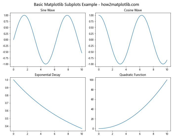
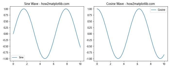
A. Line Plots (matplotlib.pyplot.plot):

Line plots are perfect for showcasing developments and adjustments over time or throughout steady variables. They’re significantly efficient for displaying knowledge with a transparent sequential relationship.

import matplotlib.pyplot as plt
import numpy as np

x = np.linspace(0, 10, 100)
y = np.sin(x)

plt.plot(x, y)
plt.xlabel("X-axis")
plt.ylabel("Y-axis")
plt.title("Easy Sine Wave")
plt.grid(True)
plt.present()

This code generates a easy sine wave. A number of traces may be added to the identical plot for comparisons. Line types, colours, markers, and legends may be personalized for enhanced readability.

B. Scatter Plots (matplotlib.pyplot.scatter):

Scatter plots are wonderful for visualizing the connection between two variables. Every knowledge level is represented as a dot, and the plot reveals correlations, clusters, and outliers.

import matplotlib.pyplot as plt
import numpy as np

np.random.seed(0)
x = np.random.rand(50)
y = 2*x + 1 + np.random.randn(50) * 0.5

plt.scatter(x, y)
plt.xlabel("X-axis")
plt.ylabel("Y-axis")
plt.title("Scatter Plot")
plt.present()

This instance exhibits a constructive correlation between x and y. Colour-coding factors primarily based on a 3rd variable provides one other dimension to the evaluation. Measurement variations can even characterize knowledge magnitude.

C. Bar Charts (matplotlib.pyplot.bar and matplotlib.pyplot.barh):

Bar charts are efficient for evaluating categorical knowledge. bar creates vertical bars, whereas barh creates horizontal bars.

import matplotlib.pyplot as plt

classes = ['A', 'B', 'C', 'D']
values = [25, 40, 15, 30]

plt.bar(classes, values)
plt.xlabel("Classes")
plt.ylabel("Values")
plt.title("Vertical Bar Chart")
plt.present()

plt.barh(classes, values)
plt.ylabel("Classes")
plt.xlabel("Values")
plt.title("Horizontal Bar Chart")
plt.present()

These charts are perfect for displaying frequencies, proportions, or comparisons throughout completely different teams. Stacked bar charts can present the contribution of subgroups to a complete.

II. Intermediate Chart Varieties:

These charts provide extra subtle methods to visualise knowledge, typically incorporating a number of variables or dimensions.

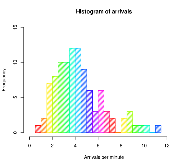
A. Histograms (matplotlib.pyplot.hist):

Histograms show the distribution of a single numerical variable. They divide the information into bins and present the frequency of knowledge factors inside every bin.

import matplotlib.pyplot as plt
import numpy as np

knowledge = np.random.randn(1000)
plt.hist(knowledge, bins=30)
plt.xlabel("Worth")
plt.ylabel("Frequency")
plt.title("Histogram")
plt.present()

Histograms are helpful for figuring out patterns like normality, skewness, and modality within the knowledge.

B. Pie Charts (matplotlib.pyplot.pie):

Pie charts present the proportions of various classes inside a complete. They’re greatest suited to a small variety of classes.

import matplotlib.pyplot as plt

labels = 'A', 'B', 'C', 'D'
sizes = [25, 30, 20, 25]

plt.pie(sizes, labels=labels, autopct='%1.1f%%', startangle=90)
plt.title("Pie Chart")
plt.axis('equal')  # Equal side ratio ensures that pie is drawn as a circle.
plt.present()

Overuse of pie charts can result in difficulties in evaluating segments, particularly when proportions are comparable.

C. Field Plots (matplotlib.pyplot.boxplot):

Field plots summarize the distribution of a numerical variable, exhibiting the median, quartiles, and outliers. They’re helpful for evaluating distributions throughout completely different teams.

import matplotlib.pyplot as plt
import numpy as np

knowledge = [np.random.normal(0, std, 100) for std in range(1, 4)]
plt.boxplot(knowledge, labels=['Group 1', 'Group 2', 'Group 3'])
plt.ylabel("Worth")
plt.title("Field Plot")
plt.present()

Field plots successfully spotlight the central tendency, unfold, and presence of outliers within the knowledge.

III. Superior Chart Varieties:

These chart varieties provide extra complicated visualization capabilities, typically leveraging a number of variables and interactive options.

A. Heatmaps (matplotlib.pyplot.imshow or seaborn.heatmap):

Heatmaps characterize knowledge as colours, the place the depth of the colour corresponds to the magnitude of the information. They are perfect for visualizing matrices or two-dimensional knowledge. Seaborn, a library constructed on prime of Matplotlib, gives enhanced performance for heatmaps.

import matplotlib.pyplot as plt
import numpy as np
import seaborn as sns

knowledge = np.random.rand(10, 10)
sns.heatmap(knowledge, annot=True, cmap="viridis")
plt.title("Heatmap")
plt.present()

Heatmaps are significantly helpful for visualizing correlation matrices, geographical knowledge, or different two-dimensional datasets.

B. 3D Plots (mpl_toolkits.mplot3d):

Matplotlib helps creating three-dimensional plots, helpful for visualizing knowledge with three variables.

import matplotlib.pyplot as plt
from mpl_toolkits.mplot3d import Axes3D
import numpy as np

fig = plt.determine()
ax = fig.add_subplot(111, projection='3d')

x = np.arange(-5, 5, 0.25)
y = np.arange(-5, 5, 0.25)
X, Y = np.meshgrid(x, y)
R = np.sqrt(X**2 + Y**2)
Z = np.sin(R)

ax.plot_surface(X, Y, Z)
plt.present()

This creates a 3D floor plot. Different 3D plot varieties embody scatter plots and wireframes.

C. Contour Plots (matplotlib.pyplot.contour):

Contour plots show traces of equal worth, helpful for visualizing features of two variables.

import matplotlib.pyplot as plt
import numpy as np

x = np.arange(-5, 5, 0.25)
y = np.arange(-5, 5, 0.25)
X, Y = np.meshgrid(x, y)
Z = np.sin(np.sqrt(X**2 + Y**2))

CS = plt.contour(X, Y, Z)
plt.clabel(CS, inline=1, fontsize=10)
plt.present()

Contour plots are generally utilized in geographical purposes and to characterize degree curves of features.

Conclusion:

Matplotlib presents a wealthy assortment of chart varieties, every serving a particular function in knowledge visualization. Selecting the suitable chart kind is essential for efficient communication of insights. This text gives a place to begin for exploring the huge capabilities of Matplotlib. Additional exploration of its documentation and superior options will unlock much more highly effective visualization strategies. Bear in mind to contemplate your viewers and the particular message you need to convey when deciding on and customizing your charts. Clear labeling, acceptable scales, and considerate shade decisions are important for creating compelling and informative visualizations.

Closure

Thus, we hope this text has supplied precious insights into Mastering Matplotlib: A Complete Information to Chart Varieties. We thanks for taking the time to learn this text. See you in our subsequent article!